Model Fit

Functional R-Squared

In functional linear regression, the model’s explanatory power can vary across the domain of the response. The plot below shows the R-squared value at each point of the electricity price curve, indicating for which hours the model explains the data well and where it may be less effective.

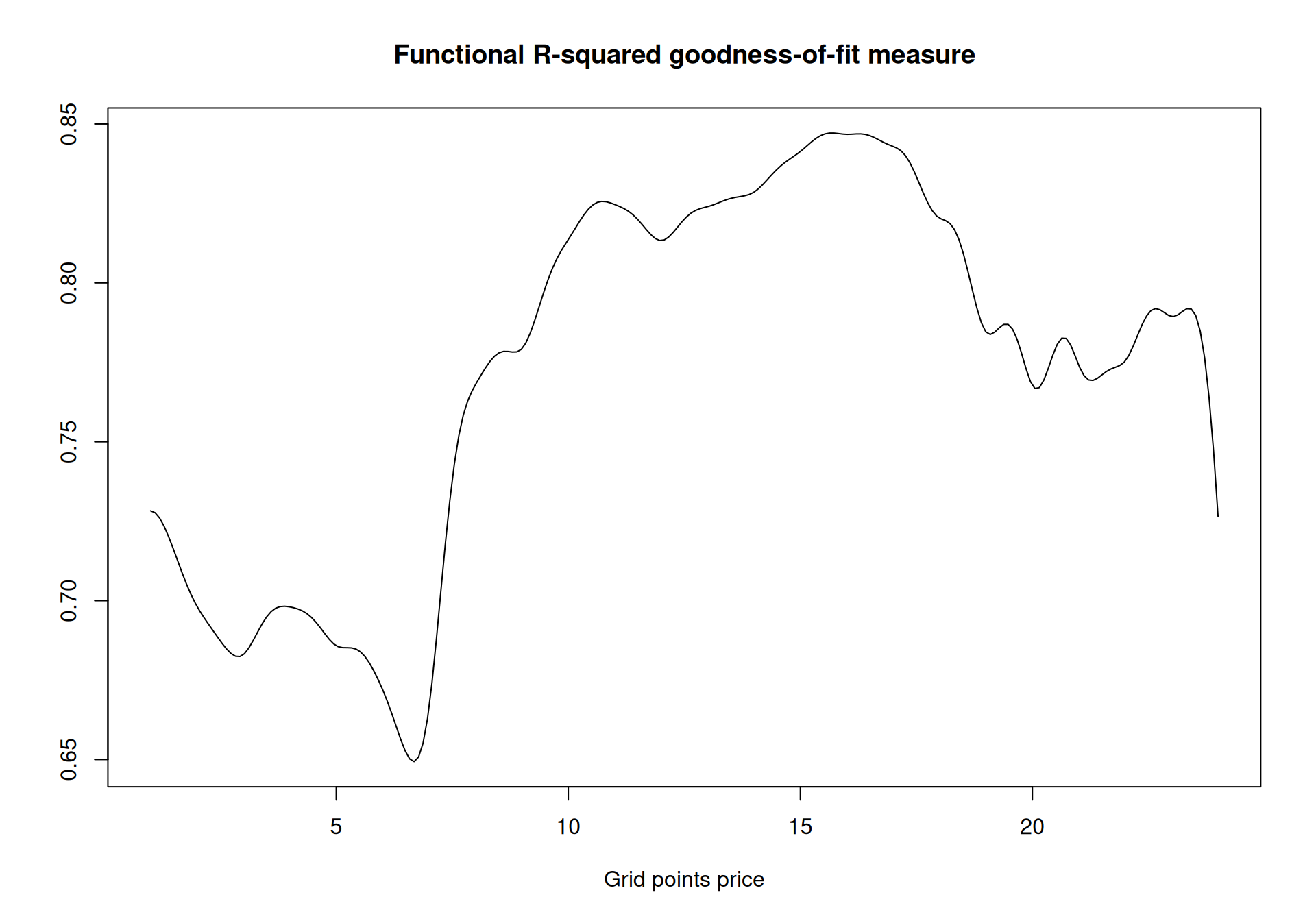
Figure 1: Functional R-squared across the 24 hours of the day.

Summary Statistics

Below are the overall fit statistics for the functional factor regression model:

## 
## Function-on-Function Linear Regression
## =======================================
## 
## Call:
## flm(formula = price ~ ., data = data, K = K_est$K, inference = TRUE)
## 
## Model Fit:
## ------------
## R-squared:           0.7729
## Adjusted R-squared:  0.7667
## RMSE:                6.3451
## MAE:                 4.0486
## 
## Model Complexity:
## ----------------
## Functional predictors factors: 38
## Number of scalar predictors: 4
## Effective degrees of freedom: 1512
## 
## Predictor Information:
## --------------------
## Monday:
##   Type: Scalar
## Tuesday:
##   Type: Scalar
## Wednesday:
##   Type: Scalar
## Thursday:
##   Type: Scalar
## price_lag1:
##   Type: Functional
##   Grid length: 240
##   Factors (K): 5
## price_lag2:
##   Type: Functional
##   Grid length: 240
##   Factors (K): 4
## price_lag5:
##   Type: Functional
##   Grid length: 240
##   Factors (K): 4
## load:
##   Type: Functional
##   Grid length: 240
##   Factors (K): 5
## load_lag1:
##   Type: Functional
##   Grid length: 240
##   Factors (K): 4
## load_lag5:
##   Type: Functional
##   Grid length: 240
##   Factors (K): 4
## windgen:
##   Type: Functional
##   Grid length: 240
##   Factors (K): 5
## windgen_lag1:
##   Type: Functional
##   Grid length: 240
##   Factors (K): 4
## windgen_lag5:
##   Type: Functional
##   Grid length: 240
##   Factors (K): 3
## 
## Visualization Options:
## -------------------
## For functional predictors:
##   plot(summary(model), predictor = 'predictor_name', which = 'beta', conf.region = TRUE)  # Plot heatmap coefficient
##   plot(summary(model), predictor = 'predictor_name', which = 'beta_3D', conf.region = TRUE)  # Plot 3D coefficient
##   plot(summary(model), predictor = 'predictor_name', which = 't')     # Plot t-values
##   plot(summary(model), predictor = 'predictor_name', which = 'p')     # Plot p-values
## 
## For scalar predictors:
##   plot(summary(model), predictor = 'predictor_name', which = 'beta')  # Plot coefficient function
## 
## For intercept:
##   plot(summary(model), predictor = 'intercept', which = 'beta')  # Plot intercept function
## 
## For goodness-of-fit measure R-squared:
##   plot(summary(model), which = 'R2')     # Plot functional R-squared